Moving Averages and Exponential Smoothing
The SMOOTH command provides features
for smoothing data by methods of moving averages and
exponential smoothing.
Consider a time series with observed values X1, X2, ..., XN. A centered 5-point moving average is obtained as:
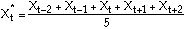 for
t = 3, ..., N
for
t = 3, ..., N-2
The number of periods used in calculating the moving average is
specified with the NMA= option on the
SMOOTH command.
The simple exponential smoothing method is based on a weighted average of current and past observations, with most weight to the current observation and declining weights to past observations. This gives the formula for the smoothed series as:
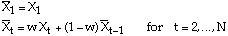
where w is a smoothing constant with a value in the range [0,1].
The value for w is specified with the WEIGHT=
option on the SMOOTH command.
Example
This example analyzes annual sales data (in thousands of dollars) of
Lydia E. Pinkham from 1931 to 1960. The data set is listed in
Newbold [1995, p. 691].
The SHAZAM commands (filename:
MASMOOTH.SHA) below
use the SMOOTH command to calculate
a centered 5-point moving average and a series smoothed by
exponential smoothing.
SAMPLE 1 30 READ SALES / BYVAR 1806 1644 1814 1770 1518 1103 1266 1473 1423 1767 2161 2336 2602 2518 2637 2177 1920 1910 1984 1787 1689 1866 1896 1684 1633 1657 1569 1390 1387 1289 GENR YEAR=TIME(1930) * Set the smoothing constant for exponential smoothing. GEN1 A=0.4 GEN1 W=1-A SMOOTH SALES / NMA=5 WEIGHT=W MAVE=MA5 * Graph the original data GRAPH SALES YEAR / LINEONLY * Graph the smoothed series SAMPLE 3 28 GRAPH MA5 YEAR / LINEONLY STOP |
The SHAZAM output can be viewed.
The results for a centered 5-point moving average are listed on the
SHAZAM output in the column MOVING-AVE
(see Newbold [1995, Table 17.12, p. 698]).
The results from exponential smoothing are listed in the column
EXP-MOV-AVE (see Newbold [1995, Table 17.16, p. 710]).
In the above SHAZAM commands, the MAVE= option
on the SMOOTH command is used to save the
moving average in the variable MA5. The
GRAPH command is then used to graph the results.
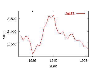
A graph of the sales data is shown below (see Newbold [1995, Figure 17.6, p. 695]).
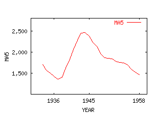
The next graph shows the series smoothed by moving averages (see Newbold [1995, Figure 17.7, p. 698]).
Forecasting with Exponential Smoothing
Exponential smoothing methods use recursive updating formula to generate forecasts. A comparison of these methods with ARIMA models is given in Mills [1990, pp. 153-163]. The recursive formula required by exponential smoothing methods can be programmed in SHAZAM. This is shown with examples from Newbold [1995, Chapter 17].
- Simple Exponential Smoothing - for nonseasonal series with no trend
- Holt-Winters Exponential Smoothing - for nonseasonal series with trend
References
Terence C. Mills, Time Series Techniques for Economists, 1990, Cambridge University Press.
Paul Newbold, Statistics for Business & Economics, Fourth Edition, 1995, Prentice-Hall.
 [SHAZAM Guide home]
SHAZAM output - Moving Averages and Simple Exponential Smoothing
 |_SAMPLE 1 30
 |_READ SALES / BYVAR
    1 VARIABLES AND       30 OBSERVATIONS STARTING AT OBS       1

 |_GENR YEAR=TIME(1930)
 |_* Set the smoothing constant for exponential smoothing.
 |_GEN1 A=0.4
 |_GEN1 W=1-A

 |_SMOOTH SALES / NMA=5 WEIGHT=W MAVE=MA5

 CENTRAL MOVING AVERAGES - PERIODS=  5 NSPAN=  1 WEIGHT= 0.600
 OBSERVATION  SALES    MOVING-AVE   SEAS&IRREG  SA(SALES   ) EXP-MOV-AVE
          1   1806.0      -------      -------       1806.0       1806.0
          2   1644.0      -------      -------       1644.0       1708.8
          3   1814.0       1710.4       1.0606       1814.0       1771.9
          4   1770.0       1569.8       1.1275       1770.0       1770.8
          5   1518.0       1494.2       1.0159       1518.0       1619.1
          6   1103.0       1426.0      0.77349       1103.0       1309.4
          7   1266.0       1356.6      0.93322       1266.0       1283.4
          8   1473.0       1406.4       1.0474       1473.0       1397.2
          9   1423.0       1618.0      0.87948       1423.0       1412.7
         10   1767.0       1832.0      0.96452       1767.0       1625.3
         11   2161.0       2057.8       1.0502       2161.0       1946.7
         12   2336.0       2276.8       1.0260       2336.0       2180.3
         13   2602.0       2450.8       1.0617       2602.0       2433.3
         14   2518.0       2454.0       1.0261       2518.0       2484.1
         15   2637.0       2370.8       1.1123       2637.0       2575.9
         16   2177.0       2232.4      0.97518       2177.0       2336.5
         17   1920.0       2125.6      0.90327       1920.0       2086.6
         18   1910.0       1955.6      0.97668       1910.0       1980.6
         19   1984.0       1858.0       1.0678       1984.0       1982.7
         20   1787.0       1847.2      0.96741       1787.0       1865.3
         21   1689.0       1844.4      0.91574       1689.0       1759.5
         22   1866.0       1784.4       1.0457       1866.0       1823.4
         23   1896.0       1753.6       1.0812       1896.0       1867.0
         24   1684.0       1747.2      0.96383       1684.0       1757.2
         25   1633.0       1687.8      0.96753       1633.0       1682.7
         26   1657.0       1586.6       1.0444       1657.0       1667.3
         27   1569.0       1527.2       1.0274       1569.0       1608.3
         28   1390.0       1458.4      0.95310       1390.0       1477.3
         29   1387.0      -------      -------       1387.0       1423.1
         30   1289.0      -------      -------       1289.0       1342.7
          1 SEASONAL FACTORS
          1   1.0000

 |_* Graph the original data
 |_GRAPH SALES YEAR / LINEONLY

        30 OBSERVATIONS
  SHAZAM WILL NOW MAKE A PLOT FOR YOU
  NO SYMBOLS WILL BE PLOTTED, LINE ONLY

 |_* Graph the smoothed series
 |_SAMPLE 3 28
 |_GRAPH MA5 YEAR / LINEONLY

        26 OBSERVATIONS
  SHAZAM WILL NOW MAKE A PLOT FOR YOU
  NO SYMBOLS WILL BE PLOTTED, LINE ONLY
 |_STOP
[SHAZAM Guide home]