Calculating a Real Interest Rate
A method for calculating a real interest rate is described in the Appendix of the paper:
Russell Davidson and James G. MacKinnon (1985), "Testing Linear and Log-linear Regressions against Box-Cox Alternatives", Canadian Journal of Economics, Vol. 18, pp. 499-517.
Suppose the nominal rate of interest is I and the expected rate of inflation is PE. The real rate of interest (R) is:
R = I - PE
An estimate of the expected rate of inflation is required.
Suppose that D is a personal expenditure
deflator (expressed as 1 in the base period). The inflation rate
between periods t and t-1 can be estimated as:
Pt = log(Dt) -
log(Dt-1)
Davidson and MacKinnon propose that a rational predictor of the inflation rate can be obtained as the predicted values from the regression:
Pt =
 1 +
2
Zt +
3 t +
et
1 +
2
Zt +
3 t +
et
where et is a random error and
Zt = 0.2 Pt-1 +
0.3 Pt-2 +
0.3 Pt-3 +
0.2 Pt-4
That is, Zt is a weighted moving average of lagged values of the inflation rate. The weights are somewhat arbitrary and they sum to 1.
Example
Quarterly data for Canada on the banks' prime lending rate and the personal
expenditure deflator were collected from the CANSIM Statistics Canada
data base for the period 1961Q1 to 1996Q3.
The data file can be viewed.
The SHAZAM commands
(filename: RATES.SHA)
for computing the real interest rate are given below.
TIME 1961 4 SAMPLE 1961.1 1996.3 * Read the CANSIM data READ (RATES.txt) DATE PDEFL RATE * Compute an inflation rate GENR PDEFL=PDEFL/100 GENR INFL=LOG(PDEFL) - LOG(LAG(PDEFL)) * Compute a weighted moving average of past inflation rates GENR INFL4=0.2*LAG(INFL) + 0.3*LAG(INFL,2) + 0.3*LAG(INFL,3) + 0.2*LAG(INFL,4) * Because of the lags, there are 5 undefined observations at the * beginning of the sample. * Adjust the sample period to exclude the undefined observations. SAMPLE 1962.2 1996.3 * Generate a time trend GENR TREND=TIME(0) * Get an expected inflation rate as the predicted values * from an OLS regression. OLS INFL INFL4 TREND / PREDICT=EINFL * Compute a real interest rate. * The factor of 400 is needed to convert quarterly rates to * annual percentage rates. GENR RR = RATE - 400*EINFL * Write the results to a data file. SAMPLE 1963.1 1996.3 FORMAT(F10.1,2F8.2) WRITE (RR.txt) DATE RATE RR / FORMAT STOP |
The SHAZAM output can be viewed.
The calculated real interest rate is written to the data file
RR.txt. This data file can then be used in
a SHAZAM program by loading the data with the command:
READ (RR.txt) DATE RATE RR / LIST |
The LIST option on the READ command
gives a complete listing of the data on the SHAZAM output file.
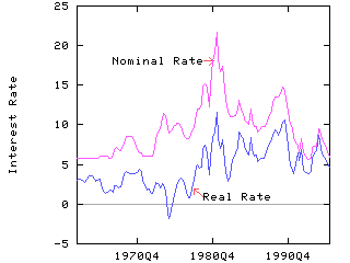
A comparison of the nominal and real interest rates for Canada is shown in the figure below.
 [SHAZAM Guide home]
SHAZAM output for computing real interest rates
 |_TIME 1961 4
 |_SAMPLE 1961.1 1996.3
 |_* Read the CANSIM data
 |_READ (RATES.txt) DATE PDEFL RATE

 UNIT 88 IS NOW ASSIGNED TO: RATES.txt
    3 VARIABLES AND      143 OBSERVATIONS STARTING AT OBS       1

 |_* Compute an inflation rate
 |_GENR PDEFL=PDEFL/100
 |_GENR INFL=LOG(PDEFL) - LOG(LAG(PDEFL))
 ..NOTE.LAG VALUE IN UNDEFINED OBSERVATIONS SET TO ZERO
 ...WARNING...ILLEGAL LOG  IN OBS.    1, VALUE REPLACED BY ZERO     .00000
 |_* Compute a weighted moving average of past inflation rates
 |_GENR INFL4=0.2*LAG(INFL) + 0.3*LAG(INFL,2) + 0.3*LAG(INFL,3) + 0.2*LAG(INFL,4)
 ..NOTE.LAG VALUE IN UNDEFINED OBSERVATIONS SET TO ZERO
 ..NOTE.LAG VALUE IN UNDEFINED OBSERVATIONS SET TO ZERO
 ..NOTE.LAG VALUE IN UNDEFINED OBSERVATIONS SET TO ZERO
 ..NOTE.LAG VALUE IN UNDEFINED OBSERVATIONS SET TO ZERO

 |_* Because of the lags, there are 5 undefined observations at the
 |_* beginning of the sample.
 |_* Adjust the sample period to exclude the undefined observations.
 |_SAMPLE 1962.2 1996.3

 |_* Generate a time trend
 |_GENR TREND=TIME(0)

 |_* Get an expected inflation rate as the predicted values
 |_* from an OLS regression.
 |_OLS INFL INFL4 TREND / PREDICT=EINFL

  OLS ESTIMATION
      138 OBSERVATIONS     DEPENDENT VARIABLE = INFL
 ...NOTE..SAMPLE RANGE SET TO:    6,  143

  R-SQUARE =    .6650     R-SQUARE ADJUSTED =    .6600
 VARIANCE OF THE ESTIMATE-SIGMA**2 =   .20972E-04
 STANDARD ERROR OF THE ESTIMATE-SIGMA =   .45795E-02
 SUM OF SQUARED ERRORS-SSE=   .28312E-02
 MEAN OF DEPENDENT VARIABLE =   .11885E-01
 LOG OF THE LIKELIHOOD FUNCTION =  548.994

 VARIABLE   ESTIMATED  STANDARD   T-RATIO        PARTIAL STANDARDIZED ELASTICITY
   NAME    COEFFICIENT   ERROR     135 DF   P-VALUE CORR. COEFFICIENT  AT MEANS
 INFL4      .87754      .5416E-01   16.20      .000  .813      .8083      .8755
 TREND     -.14247E-04  .9800E-05  -1.454      .148 -.124     -.0725     -.0893
 CONSTANT   .25416E-02  .1072E-02   2.372      .019  .200      .0000      .2139

 |_* Compute a real interest rate.
 |_* The factor of 400 is needed to convert quarterly rates to
 |_* annual percentage rates.
 |_GENR RR = RATE - 400*EINFL

 |_* Write the results to a data file.
 |_SAMPLE 1963.1 1996.3
 |_FORMAT(F10.1,2F8.2)
 |_WRITE (RR.txt) DATE RATE RR / FORMAT
 UNIT 88 IS NOW ASSIGNED TO: RR.txt
 |_STOP
[SHAZAM Guide home]